ALoDLM: Adaptively Looped Diffusion Language Models

  • Liancheng Fang (University of Illinois Chicago; equal contribution; work done at Amazon AGI)
  • Zhuowei Li (Amazon AGI; equal contribution; project lead)
  • Youngeun Kim (Korea University; work done at Amazon AGI)
  • Tianchen Zhao (Amazon AGI)
  • Rajat Koner (Amazon AGI)
  • Jiaye Wu (Amazon AGI)
  • Linghan Xu (Amazon AGI)
  • Xuanbai Chen (Amazon AGI)
  • Xiang Xu (Amazon AGI)
  • Zheng Zhang (Amazon AGI)
  • Jakub Zablocki (Amazon AGI)
  • Nishant Sankaran (Amazon AGI)
  • Yifan Xing (Amazon AGI)
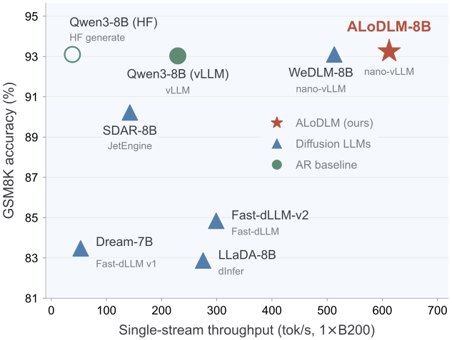
Decoding replay An illustrative side-by-side replay of one ALoDLM-8B response to a GSM8K question, paced from measured single-stream GSM8K throughput (Figure 1, right: 229.3 tok/s for vLLM-served Qwen3-8B, 612.4 tok/s for ALoDLM-8B). It needs JavaScript.

Abstract

Diffusion language models (DLMs) enable fast generation by predicting multiple tokens in parallel, yet their practical adoption remains hindered by a persistent quality gap relative to comparably sized autoregressive models. We attribute this gap to a computation–difficulty mismatch: within a partially observed sequence, some unknown tokens are readily predictable, while others require substantially more computation to resolve. Existing DLMs, however, apply uniform computational depth to every unknown position at each denoising step. We introduce ALoDLM, which replaces this uniform computation with token-adaptive latent recurrence. At each denoising step, ALoDLM iteratively refines representations in latent space, allocating computation based on token difficulty. Tokens ready to commit are fed back as discrete context, while unresolved tokens retain and refine their latent states through additional recurrent passes. To learn both token prediction and computation allocation end-to-end, we formulate token-wise computation schedules as latent variables and derive a conditional negative evidence lower bound (NELBO). We train ALoDLM at 1.7B and 8B parameter scales. Across eleven benchmarks, ALoDLM outperforms all evaluated DLMs and the corresponding autoregressive baselines in average benchmark score at both scales. Importantly, ALoDLM combines superior generation quality with fast parallel decoding, establishing a strong quality–efficiency trade-off among all evaluated autoregressive and diffusion models under optimized inference engines.

Key contributions

  • Token-adaptive looped architecture

    A looped architecture with dynamic recurrent depth: inside every denoising step, a shared recurrent core runs up to K times, the maximum recurrent depth. Easy tokens commit early and act as resolved context, while difficult tokens keep refining their accumulated latent states through additional recurrent passes.

  • Principled training objective

    Token-wise exit schedules are treated as latent variables, and a conditional NELBO learns token prediction and computation allocation end-to-end. A single-trajectory gradient estimator is unbiased for this objective; the practical recipe relaxes its KL term and adds variance reduction to stabilize training.

  • Scaling and performance

    To the best of our knowledge, ALoDLM-8B is the largest looped DLM to date. It has the best average score among all evaluated DLMs and beats its Qwen3 AR counterparts in average score over eleven benchmarks (65.5 vs 63.8 at 1.7B, 80.3 vs 78.5 at 8B), with direct SFT on a 5B-token corpus.

  • Fast decoding and test-time scaling

    On GSM8K, ALoDLM-8B delivers ≈2.7× the throughput of vLLM-served Qwen3-8B at comparable or higher accuracy. Recurrent depth is an effective test-time scaling axis, and the model learns token-dependent refinement preferences without explicit difficulty labels.

Performance overview

ALoDLM combines strong performance with fast inference.

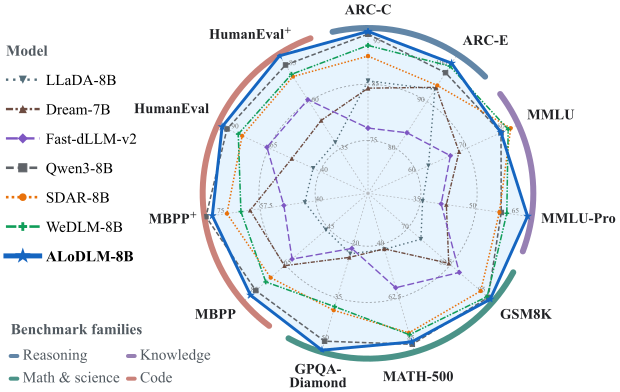
Figure 1 · left
Radar chart of 11 benchmarks: ALoDLM-8B forms the outermost polygon on most axes versus LLaDA-8B, Dream-7B, Fast-dLLM-v2, Qwen3-8B, SDAR-8B and WeDLM-8B.
Left: ALoDLM-8B outperforms all baselines on average across 11 reasoning, coding, and knowledge benchmarks.
Figure 1 · right
Scatter of GSM8K accuracy versus single-stream throughput on one B200: ALoDLM-8B sits at the top right (93.25% at 612.4 tok/s), ahead of WeDLM-8B, vLLM-served Qwen3-8B and the other diffusion LLMs.
Right: On GSM8K, ALoDLM-8B delivers ∼2.7× the throughput of vLLM-served Qwen3-8B at comparable or higher accuracy, while outperforming the diffusion baselines shown in both accuracy and throughput.

Method

ALoDLM keeps the parallel denoising of a diffusion language model and adds an inner loop to every denoising step, so that computation follows token difficulty. Part 01 shows how one step runs at inference; Part 02 shows how the model learns when to stop refining.

Motivation

The computation–difficulty mismatch

Within a single denoising step, masked positions can differ greatly in how hard they are to predict, because of intrinsic uncertainty, multi-hop reasoning, or dependence on other tokens that are still unresolved. Yet a standard DLM applies the same fixed-depth denoiser to every masked position, wasting computation on easy predictions and starving hard ones.

Confidence-based decoding helps only partly: it defers low-confidence predictions to later denoising steps, but a deferred token still gets the same fixed compute, and its latent computation is thrown away and recomputed from its mask embedding at the next step.

Schematic · Compute vs. difficulty

Masked positions in one denoising step

Example answer: She sells 16 − 3 − 4 = 9 eggs a day, so she makes $18. Masked in this step: sells, 9, eggs, so, makes, $ and 18; some are easy to predict, others (9 and 18) are hard.

Standard DLM: one fixed depth

Mismatch: easy positions get more than they need, hard ones less.

Illustrative bar chart. Every masked position gets the same fixed depth. sells, eggs, so and $ need less than that, so part of their depth is wasted. makes needs a little more, 9 clearly more and 18 the most, so they are starved.

ALoDLM: passes follow difficulty

Matched: a position keeps refining until it commits, for at most K = 4 recurrent passes.

Illustrative stacked bars on a separate scale of recurrent passes, with the same difficulty outlines. sells, eggs, so and $ commit after pass 1; makes after pass 2; 9 after pass 3; and 18 after pass 4, the maximum recurrent depth K = 4.

Principle. A DLM should maintain and refine persistent latent states for challenging tokens within each denoising step, so that computation scales with prediction difficulty.

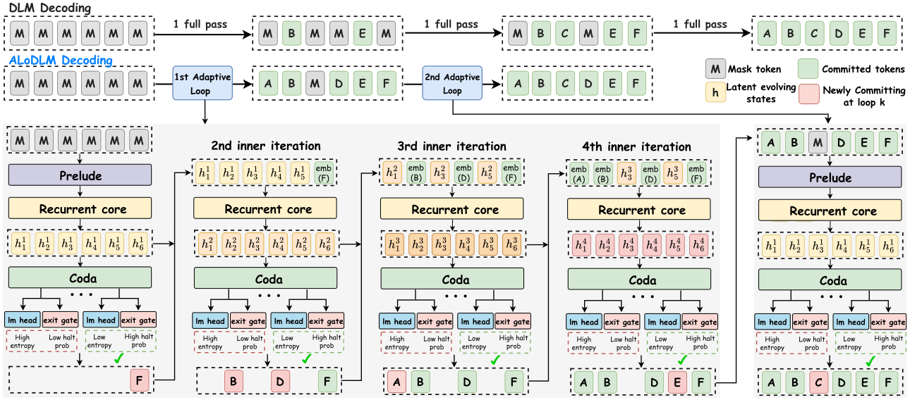
Figure 2 · Overview
Diagram comparing standard DLM decoding (fixed full passes) with ALoDLM decoding, where each denoising step runs a token-adaptive loop of Prelude, Recurrent core and Coda with per-token exit gates; confident tokens commit early and are fed back as embeddings.
Overview of ALoDLM. Standard DLMs apply a fixed-depth denoiser at each denoising step. ALoDLM introduces token-adaptive recurrence within each step: confident tokens commit early and provide discrete context, while unresolved tokens retain and refine their latent states through additional recurrent passes. Reading guide: each “Adaptive Loop” box is one denoising step and each “inner iteration” is one recurrent pass.
ALoDLM inference

Adaptive latent recurrence

A denoising step starts by encoding the partially masked sequence with the Prelude. The shared Recurrent Core then runs repeatedly; after every recurrent pass, the Coda produces a readout that feeds two heads: an LM head (a token distribution per position) and an exit gate (a halting probability).

  • Commit by confidence. After each pass, unresolved positions whose predictive entropy is at most τ are sampled and committed.
  • Feed back as context. Committed tokens re-enter the next pass as token embeddings; unresolved positions carry their latent states forward and keep refining them.
  • Stop adaptively. The exit gate’s per-pass halting probabilities accumulate into a cumulative halting probability per position; the inner loop ends when its mean over unresolved positions reaches the exit threshold q, when no unresolved positions remain, or after K = 4 passes, the maximum recurrent depth.

Latent states persist only within a step: committed tokens are written into the sequence, and the next denoising step re-initializes from it.

Inside one denoising step A step-through of recurrent passes, commitments and the exit gate on a real span of an ALoDLM-8B response with its recorded commitment passes. It needs JavaScript.

Architecture

maximum recurrent depth K = 4

ALoDLM-8B · from Qwen3-8B, 36 layers

Prelude[0, 10)
Recurrent Core [10, 26) · 16 shared layers
Coda[26, 36)

ALoDLM-1.7B · from Qwen3-1.7B, 28 layers

Recurrent Core [0, 28) · all 28 layers; Prelude = token embedding only, no Coda blocks
LM headentropy ≤ τ → commit
Exit gatemean halt ≥ q → stop

The Prelude runs once per denoising step; the Recurrent Core and the Coda readout run at every pass, and the next pass continues from the core’s output, with committed positions replaced by their token embeddings. The exit gate reads a stop-gradient copy of the readout.

Algorithm 1 and the update equations Pseudocode

One recurrent pass

(1) Core and readout
\widetilde h^{(s)} = \mathsf{Recurrent\ Core}\bigl(h^{(s-1)}\bigr), \qquad r^{(s)} = \mathsf{Coda}\bigl(\widetilde h^{(s)}\bigr), \qquad s = 1,\ldots,K
(2) LM head and per-pass halting probability
p_i^{(s)} = \operatorname{softmax}\bigl(\mathsf{LMHead}(r_i^{(s)})\bigr), \qquad \lambda_i^{(s)} = \begin{cases} \sigma\bigl(\mathsf{ExitGate}(\operatorname{sg}[r_i^{(s)}])\bigr), & s < K, \\ 1, & s = K. \end{cases}
(3) Latent feedback
h_i^{(s)} = \begin{cases} \operatorname{Emb}(\widehat y_i), & i \in \mathcal{C}^{(s)}, \\ \widetilde h_i^{(s)}, & \text{otherwise} \end{cases}
Cumulative halting probability
a_i^{(s)}=a_i^{(s-1)}+\big(1-a_i^{(s-1)}\big)\lambda_i^{(s)}

Algorithm 1 ALoDLM decoding

Input: masked sequence x, maximum depth K, entropy threshold τ, cumulative halt threshold q

  1. 1:while x contains [MASK] doOuter loop
  2. 2:U ← { i : xi = [MASK] }
  3. 3:h ← Prelude(x);  a ← 0;  C ← ∅
  4. 4:for s = 1, …, K doInner loop
  5. 5:h ← RecurrentCore(h)
  6. 6:r ← Coda(h)
  7. 7:compute pi, λi for i ∈ U by Eq. (2)
  8. 8:ai ← ai + (1 − ai)·λi,  i ∈ U
  9. 9:B ← { i ∈ U : Entropy(pi) ≤ τ }
  10. 10:ŷi ← Sample(pi),  i ∈ B
  11. 11:C ← C ∪ B;  U ← U \ B
  12. 12:hi ← Emb(ŷi),  i ∈ CCommitted tokens become context
  13. 13:if U = ∅ or meani∈U ai ≥ q then break
  14. 14:if C = ∅ thenEnsure progress
  15. 15:j ← argmini∈U Entropy(pi)
  16. 16:ŷj ← Sample(pj)
  17. 17:C ← {j}
  18. 18:xi ← ŷi,  i ∈ C
  19. 19:return x

Line 5 produces the core output \widetilde h^{(s)}; line 6 is a readout branch, and the next pass continues from the pre-Coda state. Table 1 uses a single-token quality preset: greedy token selection in place of Sample, one token committed per model pass with τ inactive, a 16-token window, and q = 0.4 (1.7B) or 0.5 (8B). Figures 1 and 3 use the parallel decoder with the entropy rule of lines 9–11.


ALoDLM training

Exit schedules as latent variables

Training learns a denoiser together with a halting policy. An exit schedule \mathbf{z} assigns every masked position i\in\mathcal{M}_t an exit depth z_i\in\{1,\ldots,K\}: token i commits after recurrent pass z_i. Together with the noisy sequence \mathbf{x}_t, a schedule fully determines one denoising step of up to K passes.

Eq. 5 Conditional NELBO
J(\theta,\phi;\mathbf{x}_t,\mathbf{y}) := \mathbb{E}_{\mathbf{z}\sim q_\phi}\Biggl[\underbrace{-\sum_{i\in\mathcal{M}_t}\log p_{\theta,i}^{(z_i)}\bigl(y_i\mid\mathbf{x}_t;\mathbf{z}\bigr)}_{\mathcal{L}_{\mathrm{traj}}(\mathbf{z})}\Biggr] + D_{\mathrm{KL}}\bigl(q_\phi\,\|\,\pi\bigr) \;\geq\; -\log p_\theta\bigl(\mathbf{y}_{\mathcal{M}_t}\mid\mathbf{x}_t\bigr)
Eq. 6 Training objective
\mathcal{L}_{\mathrm{train}}(\theta,\phi) := \mathbb{E}_{\mathbf{y}\sim p_{\mathrm{data}},\; t\sim\operatorname{Unif}[0,1],\; \mathbf{x}_t\sim q_t(\cdot\mid\mathbf{y})}\left[\frac{1}{t}\,J(\theta,\phi;\mathbf{x}_t,\mathbf{y})\right]
Eq. 7 Single-trajectory surrogate
\widehat{\mathcal{L}}_{\mathrm{sur}}(\mathbf{z}) = \frac{1}{t}\Biggl\{\mathcal{L}_{\mathrm{traj}}(\mathbf{z}) + \operatorname{sg}\!\left[\mathcal{L}_{\mathrm{traj}}(\mathbf{z}) + \log\frac{q_\phi(\mathbf{z})}{\pi(\mathbf{z})}\right]\log q_\phi(\mathbf{z})\Biggr\}
Eq. 8 Prop. 1: unbiased gradients of Eq. 6
\mathbb{E}_{\mathbf{y},t,\mathbf{x}_t,\mathbf{z}}\!\left[\nabla_{\theta,\phi}\widehat{\mathcal{L}}_{\mathrm{sur}}(\mathbf{z})\right] = \nabla_{\theta,\phi}\mathcal{L}_{\mathrm{train}}(\theta,\phi)

\mathbf{x}_t corrupted input · \mathbf{y} clean sequence · \mathcal{M}_t masked positions · q_\phi schedule distribution parameterized by the exit gate · \pi truncated-geometric prior (c = 0.4) · q_t forward masking process · \operatorname{sg} stop-gradient.

Why a bound?

Each commitment changes the context of the tokens that are still unresolved, so exit depths are modelled jointly, and summing over all exit schedules would need exponentially many separate rollouts. Instead, the exit gate parameterizes a variational distribution qϕ over schedules, and a truncated-geometric prior π with c = 0.4 favours shallow exits.
One rollout, unbiased for the objective

A schedule is sampled pass by pass during a single recurrent rollout. The denoiser is trained by ordinary backpropagation; the exit gate gets a score-function term whose detached, sequence-level cost credits each halting decision for its effect on the whole sequence. By Prop. 1 this gives unbiased gradients of the objective above. The practical recipe relaxes the KL term to keep token-wise adaptivity, reweights the denoiser loss across passes and adds an auxiliary next-token loss, so the guarantee concerns the original objective.

Lower variance, no extra passes

One rollout already yields a readout at every pass, so each token is also supervised at earlier passes, weighted by its detached exit-depth probabilities; the gate’s cost subtracts the first-pass prediction cost as a control variate. On a measured subset of 4,096 denoiser normalization parameters, removing intermediate supervision raises conditional gradient variance to 1.76×, 1.49× and 1.42× the full-method value at training steps 1k, 6.5k and 17k.

Results

ALoDLM-1.7B and ALoDLM-8B are trained from Qwen3-1.7B and Qwen3-8B by direct SFT on a 5B-token corpus, without continued pre-training, with maximum recurrent depth K = 4. All models are evaluated on eleven benchmarks with the OpenCompass protocol: native chat templates, greedy decoding, a 4,096-token generation limit, and one token per model pass under each model’s default decoding rule.

Table 1: main results Scores on eleven benchmarks at the 1.7B and 8B scales. Average score: ALoDLM-8B 80.3 vs Qwen3-8B 78.5; ALoDLM-1.7B 65.5 vs Qwen3-1.7B 63.8. The interactive table needs JavaScript.
Efficiency

Quality–efficiency trade-off

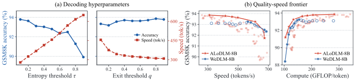
With parallel decoding on GSM8K, two thresholds set ALoDLM-8B’s operating point: the entropy threshold τ decides which tokens commit, and the exit threshold q decides how long unresolved tokens keep refining. Single-stream on one NVIDIA B200.

  • +8.5% throughputat a matched 93.25% GSM8K accuracy: 612.4 vs 564.2 tok/s against WeDLM-8B
  • 13.6% less computeat the same accuracy: 133.5 vs 154.6 estimated GFLOPs per generated token against WeDLM-8B
  • τ: 0.1 → 0.6at q = 0.5: 278.7 → 508.3 tok/s, accuracy 93.8% → 92.3% (89.9% at τ = 0.9)
  • q: 0.1 → 0.9at τ = 0.2: accuracy 93.3% → 93.8%, 455.3 → 309.0 tok/s
Figure 3 · Decoding thresholds and frontier
Left: effect of entropy threshold τ and exit threshold q on GSM8K accuracy and speed. Right: ALoDLM-8B's accuracy–speed and accuracy–compute frontiers lie above WeDLM-8B's over most of the range.
(a) Complementary roles of the entropy and halting gates. Increasing τ relaxes the commitment criterion and accelerates generation, with sharper accuracy losses at high thresholds (left). Increasing q permits deeper latent refinement, also yielding accuracy gains at lower throughput (right). These gates collectively balance parallel token commitment with adaptive refinement of unresolved tokens. (b) Adaptive recurrence improves the quality–efficiency frontier. Across most of the evaluated range, ALoDLM-8B achieves higher accuracy than WeDLM-8B at comparable throughput (left) or compute per generated token (right). Solid lines connect frontier configurations.

BibTeX

Citation for the arXiv preprint.

BibTeX
@misc{fang2026alodlmadaptivelyloopeddiffusion,
      title={ALoDLM: Adaptively Looped Diffusion Language Models},
      author={Liancheng Fang and Zhuowei Li and Youngeun Kim and Tianchen Zhao and Rajat Koner and Jiaye Wu and Linghan Xu and Xuanbai Chen and Xiang Xu and Zheng Zhang and Jakub Zablocki and Nishant Sankaran and Yifan Xing},
      year={2026},
      eprint={2610.04198},
      archivePrefix={arXiv},
      primaryClass={cs.AI},
      url={https://arxiv.org/abs/2610.04198},
}